Using da.delayed for Zarr processing: memory overhead & how to do it better?

[jluethi]

Dear dask community,

We are working on using dask for image processing of OME-Zarr files. It’s been very cool to see what’s possible with dask. Initially, we mostly did processing using the mapblocks API and things were running smoothly. But recently, we’ve started to handle some more complex cases that mapblocks doesn’t seem to handle (as far as I understand) and where we’re relying on dask.delayed & indexing. The core motivation for this is that we need to process lists of user-specified regions of interests in a large array and those regions do not necessarily have uniform sizes & positions in the array or map back to the chunks of our Zarr file or our dask array.

As an example, we may want to do something like this:

We have a list of regions of interest in a huge array, only process these small regions. If we have a dask array of 500x100kx100k, but we’re only interested in 50 cubes of 100x1000x1000 at random positions. How do we best process this? The best way we’ve found so far is using delayed functions & indexing of the dask array.

As an initial implementation of this new, more flexible approach, we’ve tried to implement a simple case that could still be done with mapblocks (see simplified code examples below). While this works, it seems to introduce slower running code and much more memory-inefficient processing. Is our approach (described below) something that should be supported and we’re doing it wrong? Or is there a better way to achieve the same goal? Does anyone have tips in how we make this more memory efficient?

---

Details:

What are we trying to achieve? Process a Zarr file by applying some functions to chunks of the data and saving it back into a new Zarr file.

We created a simplified, synthetic test example of that.

Code to generate synthetic Zarr test data:

import numpy as np
import dask.array as da


shapes = [
    (2, 2, 16000, 16000),
    (2, 4, 16000, 16000),
    (2, 8, 16000, 16000),
    (2, 16, 16000, 16000),
]

for shape in shapes:
    shape_id = f"{shape}".replace(",", "").replace(" ", "_")[1:-1]
    x = da.random.randint(0, 2 ** 16 - 1,
                          shape,
                          chunks=(1, 1, 2000, 2000),
                          dtype=np.uint16)
    x.to_zarr(f"data_{shape_id}.zarr")

Code to process the data using a mapblocks approach

SIZE = 2000
# Function which increases value of each index in 
# a SIZExSIZE image by one (=> pseudo-processing)
def shift_img(img):
    return img.copy() + 1

def process_zarr_mapblocks(input_zarr):
    out_zarr = f"out_{input_zarr}"
    data_old = da.from_zarr(input_zarr)

    n_c, n_z, n_y, n_x = data_old.shape[:]
    dtype = np.uint16
    print(f"Input file: {input_zarr}")
    print(f"Output file: {out_zarr}")
    print("Array shape:", data_old.shape)
    print("Array chunks:", data_old.chunks)
    print(f"Image size: ({SIZE},{SIZE})")

    data_new = data_old.map_blocks(
        shift_img,
        chunks=data_old.chunks,
        meta=np.array((), dtype=dtype),
    )            
    
    # Write data_new to disk (triggers execution)
    data_new.to_zarr(out_zarr)

    # Clean up output folder
    shutil.rmtree(out_zarr)

New, more flexible index-based approach to process the data

SIZE = 2000
# Function which increases value of each index in 
# a SIZExSIZE image by one (=> pseudo-processing)
def shift_img(img):
    return img.copy() + 1

def process_zarr(input_zarr):
    out_zarr = f"out_{input_zarr}"
    data_old = da.from_zarr(input_zarr)
    data_new = da.empty(data_old.shape,
                        chunks=data_old.chunks,
                        dtype=data_old.dtype)

    n_c, n_z, n_y, n_x = data_old.shape[:]

    print(f"Input file: {input_zarr}")
    print(f"Output file: {out_zarr}")
    print("Array shape:", data_old.shape)
    print("Array chunks:", data_old.chunks)
    print(f"Image size: ({SIZE},{SIZE})")


    for i_c in range(n_c):
        for i_z in range(n_z):
            for i_y in range(0, n_y - 1, SIZE):
                for i_x in range(0, n_x - 1, SIZE):
                    # Need to do this in 2 steps to avoid a
                    # TypeError: Delayed objects of unspecified length have no len()
                    new_img = delayed_shift_img(data_old[i_c, i_z, i_y:i_y+SIZE, i_x:i_x+SIZE])
                    data_new[i_c, i_z, i_y:i_y+SIZE, i_x:i_x+SIZE] = da.from_delayed(new_img,
                                                                                     shape=(SIZE, SIZE),
                                                                                     dtype=data_old.dtype)


    # Write data_new to disk (triggers execution)
    data_new.to_zarr(out_zarr)

    # Clean up output folder
    shutil.rmtree(out_zarr)

(for these tests, we go over the same regions as with mapblocks, but we've also tested the more generic approach)

Code to run the example based on different synthetic Zarr datasets & measure memory usage

input_zarrs = ['data_2_2_16000_16000.zarr', 'data_2_4_16000_16000.zarr', 'data_2_8_16000_16000.zarr', 'data_2_16_16000_16000.zarr']
for input_zarr in input_zarrs:
    interval = 0.1
    mem = memory_usage((process_zarr_mapblocks, (input_zarr,)), interval=interval)
    #mem = memory_usage((process_zarr, (input_zarr,)), interval=interval)
    time = np.arange(len(mem)) * interval
    mem_file = "log_memory_" + input_zarr.split(".zarr")[0] + "_mapblocks.dat"
    #mem_file = "log_memory_" + input_zarr.split(".zarr")[0] + "_.dat"
    print(mem_file)
    np.savetxt(mem_file, np.array((time, mem)).T)

------

What we observe

Using dask 2022.7.0 and python 3.9.12

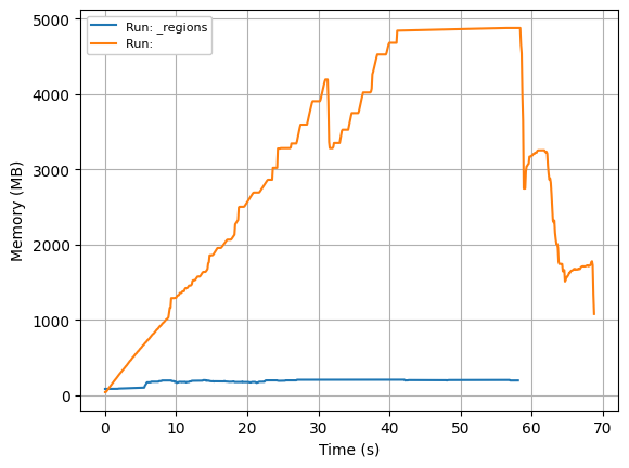
For the mapblocks approach (full lines) to process the data, the runtime scales with the dataset size, but memory usage remains stable at < 1GB.

For the indexing approach (dotted lines), processing time also scales with the size of the dataset (a bit slower in this synthetic test case, but that seems to vary depending on test cases), but memory usage scales super-linear. While the small datasets (2, 2, 16k, 16k) & (2, 4, 16k, 16k) also use < 1 GB of memory, (2, 8, 16k, 16k) uses > 1 GB and (2, 16, 16k, 16k) peaks at almost 5 GB of memory usage.

Potential explanation:
When using our indexing approach, it appears that nothing is written to the zarr file until the end. That would explain why memory accumulates. But how do we change that? With the same to_zarr call in the mapblocks example, data is continuously written to the zarr file. Why isn’t this working in our delayed/indexing approach?

We describe our approach and the memory issue in further detail here: [ROI] Memory and running time for ROI-based illumination correction · Issue #131 · fractal-analytics-platform/fractal · GitHub

Tl;dr: How do we best process a Zarr file using dask in arbitrary chunks and how do we ensure that dask continuously writes to disk during the processing, not just at the end of processing?

---

Side note: I’ve started to test this in the 2022.08.0 version of dask in recent days and, while memory usage still scales super-linear (in a slightly different pattern), performance is about 30x slower with the indexing approach. I’ll open a separate dask issue for this performance slow-down between the dask releases. But for testing this, we were on 2022.07.0 only.

[jluethi]

Because I can only have 2 links per post, here are some additional ones:

Context of the project we’re working on:

GitHub - fractal-analytics-platform/fractal: Fractal is a framework to...

Context for why we need to process in those defined regions:

Field of view parallelization via OME-NGFF ROI tables

[jluethi]

I reported the 2022070 vs. 2022080 performance differences for our indexing workflow here: Performance hit with da.delayed processing in dask 2022080 vs 2022070 · Issue #9389 · dask/dask · GitHub
The mapblocks workflow is not affected and performs the same in both cases.

[jluethi]

Just realized the example code was missing the definition of the delayed function (thanks Guillaume!):
It is the following: delayed_shift_img = dask.delayed(shift_img)
(and requires importing dask separately as in import dask)

[jni]

I’m just spitballing here, but:

• when creating the task graph, dask doesn’t know which indexes are getting set, only that some index needs to be set. (Is this true?) That is, it doesn’t know at compute time that an index in data_new will not be updated by a later operation.
• therefore, it waits until all the operations are completed before writing to zarr, because index [0, 0] might still be modified later.

Having said this, I would therefore expect the indexing approach to take much longer than map_blocks, because there should be exactly zero parallelisation — dask should want to process the operations in sequence. Is that what happens? Do you see a difference in the number of compute cores being used between the approaches?

btw, TIL that you can make writeable dask arrays with da.empty!

[jluethi]

Thanks for the ideas @jni . I was also worried on that front initially, because that would make our approach quite unviable. I had a look at the dask graph for an even smaller case though (just 4 blocks to be processed, in the same structure, i.e. 2, 2, 2000, 2000 with 2000x2000 chunks) and to me, it looks like the dask graph actually handles this well.
Here it is colored by execution order, looking as if it would process chunk by chunk and save them separately.

Code below on how to generate this, with compute=False in the to_zarr call so we just get the dask graph, not yet the output.

Code to generate the graph

input_zarr = 'data_2_2_2000_2000.zarr'
out_zarr = f"out_{input_zarr}"
data_old = da.from_zarr(input_zarr)
data_new = da.empty(data_old.shape,
                    chunks=data_old.chunks,
                    dtype=data_old.dtype)

n_c, n_z, n_y, n_x = data_old.shape[:]

print(f"Input file: {input_zarr}")
print(f"Output file: {out_zarr}")
print("Array shape:", data_old.shape)
print("Array chunks:", data_old.chunks)
print(f"Image size: ({SIZE},{SIZE})")


for i_c in range(n_c):
    for i_z in range(n_z):
        for i_y in range(0, n_y - 1, SIZE):
            for i_x in range(0, n_x - 1, SIZE):
                new_img = delayed_shift_img(data_old[i_c, i_z, i_y:i_y+SIZE, i_x:i_x+SIZE])
                data_new[i_c, i_z, i_y:i_y+SIZE, i_x:i_x+SIZE] = da.from_delayed(new_img,
                                                                                 shape=(SIZE, SIZE),
                                                                                 dtype=data_old.dtype)

# Setting compute to False so it just generates the graph, without having to execute it
output = data_new.to_zarr(out_zarr, compute=False)

We can look at the same graph with the operations marked and see it goes from from_zarr to store-map.

Thus, to me it looks like dask does figure out which indices are set when and creates a fitting graph. And the graph looks like it should parallelise well. But maybe I’m also reading the graph wrong?
And it’s hard to visualize such a graph for a much bigger example. But the data_2_2_16000_16000.zarr example still generates a graph were the colors are sorted and look distinct, thus I’d assume it can run different parts separately.

But in all those tests, it never writes to the zarr file before it’s finished processing, so I wanted to debug this further. I profiled the runtime & memory usage with to_zarr(compute=False). My thinking was that if I run this with compute=False, it will build the dask graph, but not do any of the computation and not use much memory. That apparently is a wrong assumption. This is the run profile vs. compute=True (in orange):

So my assumption that setting compute=False would not make my dask graph in this scenario compute anything was wrong. This made me suspicious that we were falling for this issue here that Guillaume Witz suggested on Zulip of calling delayed too much: Best Practices — Dask documentation

Thus, I looked into the store function that dask uses to save to Zarr.
That function says: “It stores values chunk by chunk so that it does not have to fill up memory.” (=> what we want!) The function also calls Delayed on the output if compute is False. Thus, I tested running this without using dask.delayed in my main code. Just using this in the loop:

data_new[i_c, i_z, i_y:i_y+SIZE, i_x:i_x+SIZE] = data_old[i_c, i_z, i_y:i_y+SIZE, i_x:i_x+SIZE]

Red & orange: Removing the to_zarr call => runs very briefly, but doesn’t save anything. But just our code above, with or without us calling delayed on our shift_img function, does not trigger much computation if there is no to_zarr in the end.
But whether I remove the delayed call in our function or not, it runs at the same speed & same memory usage. And when to_Zarr compute is set to False, it just ends around 55s (after the memory peak).

---

In conclusion, I think I’m still were I started. @jni Would you agree with how I read the graphs that the dask graph is actually split nicely?

Also, I started having a look at using the regions property of to_zarr (to force it to really write one region at a time). See here dask.array.to_zarr — Dask documentation or here Adds region to to_zarr when using existing array by chrisroat · Pull Request #8590 · dask/dask · GitHub
Unfortunately, the documentation of it is quite sparse and I haven’t managed to figure out whether that’s a bad thing to use or I’m just using it wrong. It would be one hope to really force dask to write single regions at a time to disk, if I understand its intended use correctly.

[jni]

Can you show me what the task graph for this tiny example looks like with the map_blocks approach? I’m worried about the single box at the bottom — is there always such a box? In the simple case of a da.random.random((10, 10), chunks=(5, 5)) → to_zarr, the graph components are disjoint:

[jluethi]

Interesting question @jni . When using the mapblocks example from the original post and visualizing it, it has the same connectivity, but is much more concise. Also using the smallest 2_2_2000_2000 example like for the graphs above, I get this:

In general, I’m not sure whether we’d need to separate the data into distinct junks before we start the dask graph. At least in the mapblocks scenario, it is not required. And the resulting dask graph looks like (a shorter version of) the graph we get when doing indexing (which is why I was expecting this indexing approach to work initially).

[jluethi]

Regarding whether the graph connects at the bottom, we can also avoid that (thanks @tcompa for the reminder!). By using inline_array=True when reading the zarr file, we split up the reading of the array in distinct chunks. Unfortunately, it doesn’t change any of the results.

This is how the graph looks with inline_array=True:

And this is the performance, basically equal for inline_array=True (with or without using the delayed call in our function) to the original performance in green (from the top post). And all much worse than the mapblocks (see original post):

[jluethi]

I think I have it! It appears that using the region parameter of to_zarr properly does the trick and reduces memory usage drastically!
Thanks a lot Davis Bennett for the support in how to use dask & how to use the regions parameter!

I’ll do some further tests and report some working code a bit later

[jluethi]

For completeness, here’s the full version of our current solution:

The essential part was to split up the whole process into single tasks per chunk and use the region parameter in to_zarr to just write that specific ROI to the zarr file for any given task.
Also, when calling to_zarr with compute=False (in order to generate all the dask tasks that we can then process), it’s not necessary anymore to use dask.delayed on the function (and also in other tests, when the output is a to_zarr, it’s not actually required to call dask.delayed on the function, because the to_zarr part already enforces the computation to be delayed).

Here is the code using region properly

def process_zarr_regions(input_zarr, inplace=False, overwrite=True):
    if inplace and not overwrite:
        raise Exception('If zarr is processed in place, overwrite needs to be True')

    out_zarr = f"out_{input_zarr}"
    data_old = da.from_zarr(input_zarr)

    # Prepare output zarr file
    if inplace:
        new_zarr = zarr.open(input_zarr)
    else:
        new_zarr = zarr.create(
            shape=data_old.shape,
            chunks=data_old.chunksize,
            dtype=data_old.dtype,
            store=da.core.get_mapper(out_zarr),
            overwrite=overwrite,
        )
    n_c, n_z, n_y, n_x = data_old.shape[:]

    print(f"Input file: {input_zarr}")
    print(f"Output file: {out_zarr}")
    print("Array shape:", data_old.shape)
    print("Array chunks:", data_old.chunks)
    print(f"Image size: ({SIZE},{SIZE})")

    tasks = []
    regions = []
    for i_c in range(n_c):
        for i_z in range(n_z):
            for i_y in range(0, n_y - 1, SIZE):
                for i_x in range(0, n_x - 1, SIZE):
                    regions.append((slice(i_c, i_c+1), slice(i_z, i_z+1), slice(i_y,i_y+SIZE), slice(i_x,i_x+SIZE)))
    
    for region in regions:
        data_new = shift_img(data_old[region])
        task = data_new.to_zarr(url=new_zarr, region=region, compute=False, overwrite=overwrite)
        tasks.append(task)

    # Compute tasks sequentially
    # TODO: Figure out how to run tasks in parallel where save => batching
    # (where they don't read/write from/to the same chunk)
    for task in tasks:
        task.compute()

Here are how the memory profiles compare for the largest example (the 2, 16, 16000, 16000 case, it scales as before for the smaller examples):

Summary:

1. Our initial indexing approach was the worst (blue line) => long runtime & high memory usage
2. The mapblocks approach is a mix: Much shorter runtime, intermediate memory usage
3. The new region approach runs all tasks sequentially. Thus, runtime is comparable to the initial indexing, memory usage is very low (even lower than mapblocks)
4. There is a bit of variability between runs and saving to a new zarr file may be slightly faster than overwriting the ROIs in the existing file. But the overhead is quite acceptable for our use-case.

---

Downsides compared to the mapblocks implementation:
We don’t have dask handling the question of assigning overlapping indices. For what we are planning to do, we don’t want to write the same pixel position multiple times. But we need to do that handling.
Also, using an indexing approach does have some overhead that scales with the number of ROIs. When not doing the compute, runtime scales up from 1s (for 256 ROIs in the 2, 2, 16000, 16000 case) to ~6s (for 2048 ROIs in the 2, 16, 16000, 16000 case), while mapblocks just seems to vary a bit, but likely would stay constant even for higher number of ROIs.

For our use-case, we will probably mostly have dozens to hundreds of ROIs, so that should be fine. But if one applies this logic to arbitrary number of ROIs, scaling isn’t great.

---

Room for improvement:
I’m currently running all the ROIs sequentially. One could come up with a way to batch them and I’d assume that this would decrease runtime & increase memory usage. Such batching is non-trivial though, because we can only batch tasks that don’t need to write to the same underlying chunk in the zarr array, so may be a bit tricky to calculate this. Thus, achieving the same runtimes as mapblocks will not be trivial (but if we find a good way to do this, we can tune the runtime vs. memory usage trade-off explicitly).

---

Things to be tests
We’ll now need to test implementing this approach for our real-world use-cases again. Typically, the data is a bit bigger, though we normally have fewer ROIs (~100). The actual run functions will be doing much more than our dummy function at the moment, so the overhead may become negligible, but we’ll need to test that. Curious to see how this performs, whether we can use the inplace version and how easy it will be to do some parallelization.

---

In conclusion: This is the solution we need for our use-case of arbitrary ROIs. Splitting the processing into distinct tasks and using region in to zarr enables this use case. There are some trade-offs with complexity, overhead & runtime (but those trade-offs should be worth it for the ROI flexibility we’re gaining in our use-case).

---

Thanks a lot Davis Bennett for the support, everyone else on the napari Zulip & @jni here on the forum as well!

PS: Learning for anyone attempting this as well: The region property only takes tuples of slice, not e.g. list, single integers or such.

[d-v-b]

Glad I could help, @jluethi

[beder]

What memory profiler library was used to create the graphs in this post?

Thank you.

[jluethi]

Hey @beder

For the memory profiling, we used memory_profiler:

from memory_profiler import memory_usage
import numpy as np

if __name__ == "__main__":
    input_zarr = sys.argv[1]
    interval = 0.1
    mem = memory_usage((process_zarr, (input_zarr,)), interval=interval)
    time = np.arange(len(mem)) * interval
    mem_file = "log_memory_" + input_zarr.split(".zarr")[0] + ".dat"
    print(mem_file)
    np.savetxt(mem_file, np.array((time, mem)).T)

For plotting, it’s just some custom matplotlib code:

import numpy as np
import matplotlib.pyplot as plt

for n_z in [2, 4, 8, 16]:
    f = f"log_memory_data_2_{n_z}_16000_16000.dat"
    t, mem = np.loadtxt(f, unpack=True)
    plt.plot(t, mem, label=f"shape=(2,{n_z},16k,16k)")
    print(f, np.max(mem))

plt.xlabel("Time (s)")
plt.ylabel("Memory (MB)")
plt.legend(fontsize=8, framealpha=1)
plt.grid()
plt.savefig("fig_memory.png", dpi=256)

See the full details here: [ROI] Memory and running time for ROI-based illumination correction · Issue #27 · fractal-analytics-platform/fractal-tasks-core · GitHub

[beder]

Thank you for the quick reply! I have read through your example above to take ideas from while building out a similar workflow to chunk and process Sentinel-2 satellite data.

[jluethi]

Cool!

We haven’t really come back to this so far, because our solution of using regions and explicit compute calls works decently. It keeps memory usage very stably in check. It does not parallelize as much as would be possible with the fancier dask graphs we tried in the beginning, but we’re mostly IO limited anyway. Thus, additional parallelization hasn’t been a core priority.

I still think it should probably be possible to make more use of the parallelization while staying in the memory envelope though when IO is not limiting.